Studios for interactive analysis
Studios runs interactive analysis environments — Jupyter notebooks, an R-IDE, Visual Studio Code, and Xpra remote desktops — on your Seqera Platform compute environments, with your cloud data mounted directly into each session.
In this tutorial, you'll set up a compute environment and mount public pipeline data, then build a Studio for each environment type:
- Jupyter: visualize protein structures predicted by nf-core/proteinfold.
- R-IDE: explore RNA-Seq differential expression results in a Shiny app.
- Xpra: view genetic variants from the 1000 Genomes Project in IGV desktop.
- VS Code: create a Nextflow development environment with nf-core tools.
Each example stands alone. Complete the setup once, then jump to the environment you use.
Before you begin
You need:
- At least the Maintain workspace user role to create and configure Studios.
- Valid credentials for your cloud storage account and compute environment.
- Data Explorer enabled in your workspace.
The library and package versions pinned in these examples may become outdated over time and lead to unexpected results.
Set up a compute environment
The examples in this tutorial use an AWS Batch compute environment. Studios also supports AWS Cloud, Azure Cloud, and Google Cloud compute environments — see Add a Studio for requirements per platform.
If you don't have an existing AWS Batch compute environment, create one with the following attributes:
- Region: To minimize costs, create the compute environment in the same region as your data. Each example below lists the region of its public dataset.
- Provisioning model: Use On-demand EC2 instances.
- Do not enable Use Fargate for head job. Studios does not support AWS Fargate.
- At least 2 available CPUs and 8192 MB of RAM. The VS Code example needs 4 CPUs and 16384 MB of RAM.
Studio sessions compete for resources with pipeline runs on a shared compute environment. Ensure the compute environment has sufficient resources to run both.
Add public data with Data Explorer
Each example mounts a public dataset into the Studio session:
| Example | Bucket path | Region |
|---|---|---|
| Jupyter | s3://nf-core-awsmegatests/proteinfold/results-9bea0dc4ebb26358142afbcab3d7efd962d3a820 | eu-west-1 |
| R-IDE | s3://nf-core-awsmegatests | eu-west-1 |
| Xpra | s3://1000genomes | us-east-1 |
| VS Code | s3://ngi-igenomes/test-data/ | eu-west-1 |
To add a bucket to your workspace:
- From the Data Explorer tab, select Add cloud bucket.
- Specify the bucket details:
- Provider: AWS
- Bucket path: the path from the table above
- A unique Name for the bucket, such as
nf-core-awsmegatests - Credentials: Public
- An optional bucket Description
- Select Add.
To analyze your own pipeline results instead, add the cloud bucket that contains them. See Add a cloud bucket.
Jupyter: Visualize protein structure predictions
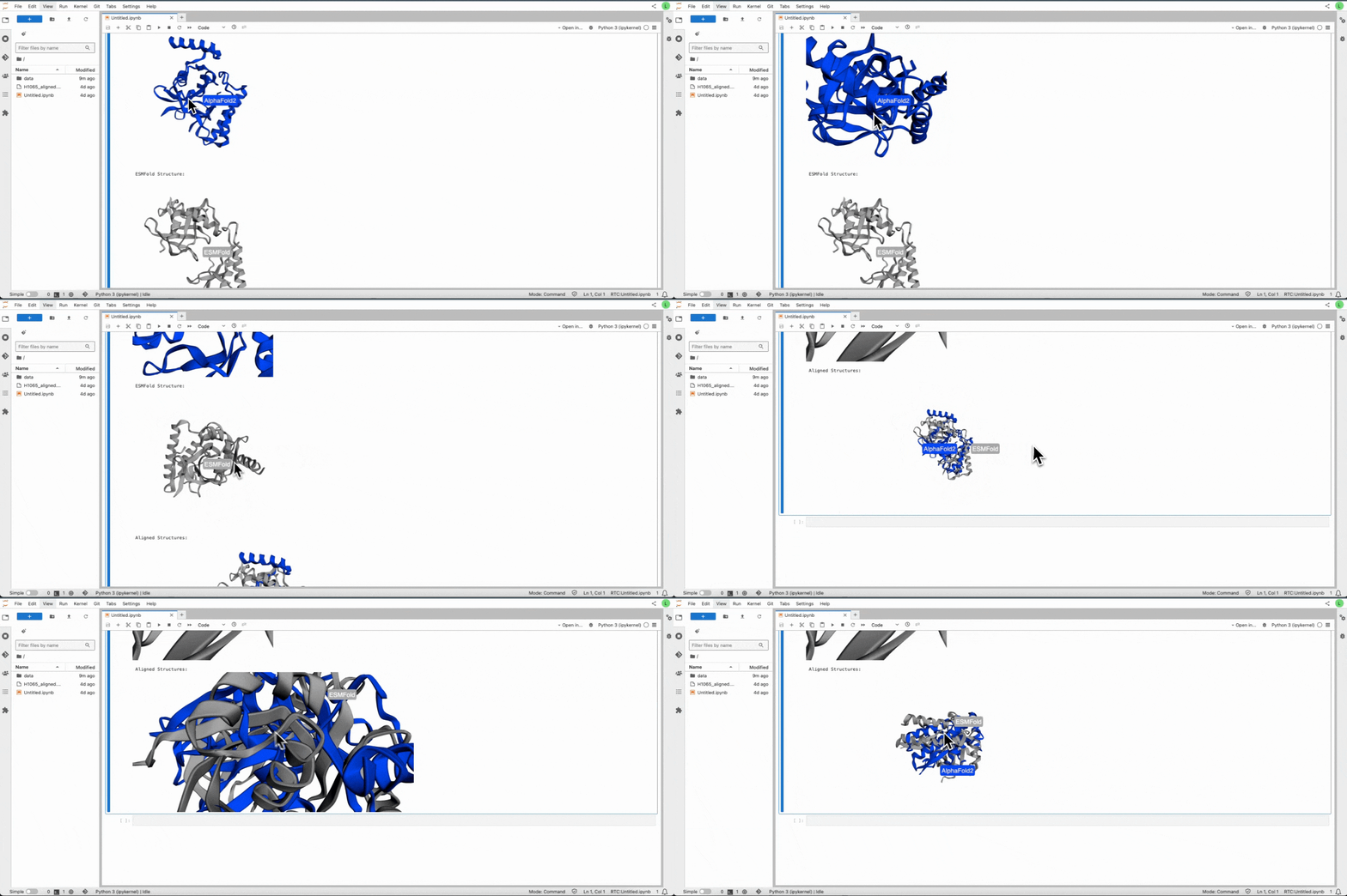
Jupyter notebooks enable interactive analysis with Python libraries and tools. In this example, you use Py3DMol to visualize and compare protein structures produced by nf-core/proteinfold, rendering interactive composite 3D images of the H1065 sequence from the nf-core AWS megatests public dataset. The same script works with the results of your own nf-core/proteinfold runs.
Create the Jupyter Studio
-
From the Studios tab, select Add Studio.
-
In the Compute & Data tab:
- Select your AWS Batch compute environment.
- Optional: Enter CPU and memory allocations. The default values are 2 CPUs and 8192 MB memory (RAM).
- Mount the proteinfold bucket you added with Data Explorer, or the results directory of your own nf-core/proteinfold run.
-
In the General config tab:
- Select the latest Jupyter container image template from the list.
- Optional: Enter a unique name and description for the Studio.
- Check Install Conda packages and paste the following into the YAML textfield:
channels:
- schrodinger
- conda-forge
- bioconda
dependencies:
- python=3.10
- conda-forge::libgl
- pip
- pip:
  - biopython==1.85
  - mdtraj==1.10.3
- py3dmol==2.4.2 -
Select Add and start, then select Connect in the options menu to open the session in a new browser tab when it is running.
Installing Conda packages builds a custom container environment for your session. For the package syntax, prerequisites, and other ways to customize a Studio — including your own container images — see Custom environments.
Visualize protein structures
The following Python script creates a composite interactive 3D image of the structures predicted by AlphaFold2 and ESMFold in contrasting colors. It aligns the mobile structure to the reference structure with Biopython's Superimposer, then renders individual and combined interactive views with Py3DMol.
Run the script in your Jupyter notebook:
Full Python script
import py3Dmol
from IPython.display import display
from Bio import PDB
from Bio.PDB import Superimposer
import numpy as np

# Keep file paths unchanged to visualize structures of the H1065 sequence in nf-core AWS megatests.
# Update file paths (to PDB files) to visualize structures of your own nf-core/proteinfold output data.
alphafold2_multimer_standard = "/workspace/data/nf-core-awsmegatests-proteinfold-h1065/mode_alphafold2_multimer/alphafold2/standard/H1065.alphafold.pdb"
esmfold_multimer = "/workspace/data/nf-core-awsmegatests-proteinfold-h1065/mode_esmfold_multimer/esmfold/H1065.pdb"

def align_structures(ref_pdb_path, mobile_pdb_path):
    """Align mobile structure to reference structure and return aligned coordinates"""
    # Set up parser
    parser = PDB.PDBParser()

    # Load structures
    ref_structure = parser.get_structure("reference", ref_pdb_path)
    mobile_structure = parser.get_structure("mobile", mobile_pdb_path)

    # Get lists of C-alpha atoms from both structures
    ref_atoms = []
    mobile_atoms = []

    for model in ref_structure:
        for chain in model:
            for residue in chain:
                if 'CA' in residue:
                    ref_atoms.append(residue['CA'])

    for model in mobile_structure:
        for chain in model:
            for residue in chain:
                if 'CA' in residue:
                    mobile_atoms.append(residue['CA'])

# Align structures using Superimposer
super_imposer = Superimposer()
super_imposer.set_atoms(ref_atoms, mobile_atoms)
super_imposer.apply(mobile_structure.get_atoms())

# Save aligned structure
io = PDB.PDBIO()
io.set_structure(mobile_structure)
aligned_pdb_path = "./"+mobile_pdb_path.split("/")[-1].replace('.pdb', '_aligned.pdb')
io.save(aligned_pdb_path)

return aligned_pdb_path

def create_structure_view(pdb_path, color, width=400, height=400, label=None):
    """Create a view for a single structure"""
    view = py3Dmol.view(width=width, height=height)

    with open(pdb_path, 'r') as f:
        pdb_data = f.read()
    view.addModel(pdb_data, "pdb")
    view.setStyle({'model': -1}, {'cartoon': {'color': color}})
    view.zoomTo()

    if label:
        view.addLabel(label, {
            'position': {'x': 0, 'y': 0, 'z': 0},
            'backgroundColor': color,
            'fontColor': 'white'
        })

    return view

def visualize_structures(pdb1_path, pdb2_path):
    # Align the second structure to the first
    aligned_pdb2_path = align_structures(pdb1_path, pdb2_path)

    # Create three separate views
    view1 = create_structure_view(pdb1_path, 'blue', label="AlphaFold2")
    view2 = create_structure_view(aligned_pdb2_path, 'darkgrey', label="ESMFold")

    # Create combined view
    view3 = py3Dmol.view(width=800, height=400)

    # Load and display first structure (AlphaFold2)
    with open(pdb1_path, 'r') as f:
        pdb1_data = f.read()
    view3.addModel(pdb1_data, "pdb")
    view3.setStyle({'model': -1}, {'cartoon': {'color': 'blue'}})

    # Load and display aligned second structure (ESMFold)
    with open(aligned_pdb2_path, 'r') as f:
        pdb2_data = f.read()
    view3.addModel(pdb2_data, "pdb")
    view3.setStyle({'model': 1}, {'cartoon': {'color': 'darkgrey'}})

    # Set up the combined view
    view3.zoomTo()

    # Add labels for combined view
    view3.addLabel("AlphaFold2", {'position': {'x': -20, 'y': 0, 'z': 0}, 'backgroundColor': 'blue', 'fontColor': 'white'})
    view3.addLabel("ESMFold", {'position': {'x': 20, 'y': 0, 'z': 0}, 'backgroundColor': 'darkgrey', 'fontColor': 'white'})

    return view1, view2, view3

# Visualize the structures
view1, view2, view3 = visualize_structures(alphafold2_multimer_standard, esmfold_multimer)

# Display all views
print("AlphaFold2 Structure:")
view1.show()
print("\nESMFold Structure:")
view2.show()
print("\nAligned Structures:")
view3.show()
R-IDE: Explore RNA-Seq differential expression results
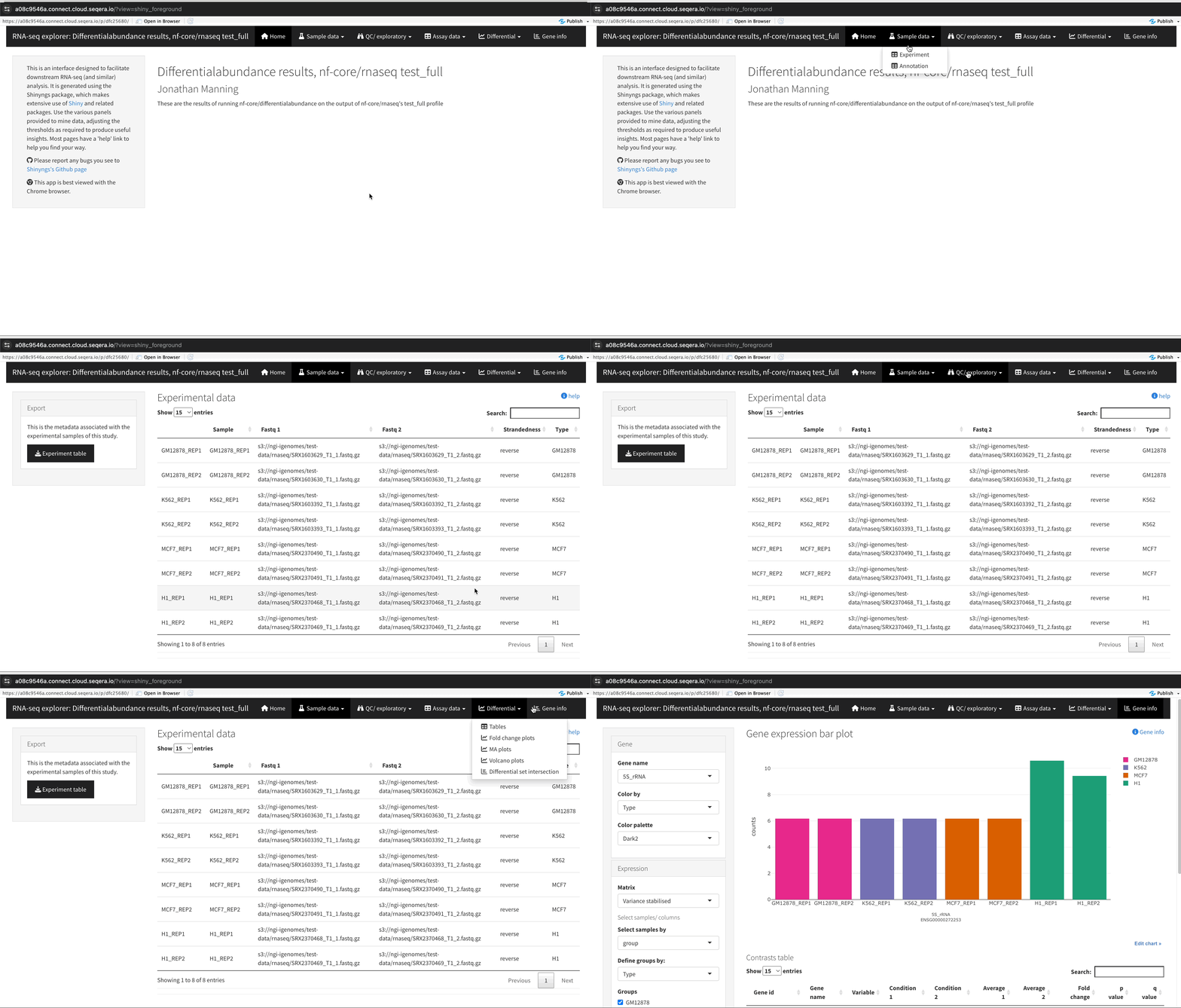
An R-IDE enables interactive analysis with R libraries and tools. In this example, you deploy ShinyNGS, a Shiny web app created by members of the nf-core community, to explore public RNA sequencing data that was processed by nf-core/rnaseq to quantify gene expression, followed by nf-core/differentialabundance to derive differential expression statistics.
Create the R-IDE Studio
- From the Studios tab, select Add Studio.
- In the Compute & Data tab:
- Select your AWS Batch compute environment.
- Optional: Enter CPU and memory allocations. The default values are 2 CPUs and 8192 MB memory (RAM).
- Mount the nf-core AWS megatests bucket you added with Data Explorer, or the results directory of your own nf-core/differentialabundance run.
- In the General config tab:
- Select the latest R-IDE container image template from the list.
- Optional: Enter a unique name and description for the Studio.
- Select Add and start, then select Connect in the options menu to open the session in a new browser tab when it is running.
Deploy the ShinyNGS app
The following R script installs the prerequisite packages, downloads the RDS input file, and launches the app's plots, heatmaps, and tables. To use your own nf-core/rnaseq and nf-core/differentialabundance results, replace the download URL in step 2:
R script individual steps
-
Configure the R-IDE session with installed packages, including ShinyNGS:
if (!require("BiocManager", quietly = TRUE))
  install.packages("BiocManager")

BiocManager::install(version = "3.20", ask = FALSE)
BiocManager::install(c("SummarizedExperiment", "GSEABase", "limma"))

install.packages(c("devtools", "matrixStats", "rmarkdown", "markdown"))
install.packages("shiny", repos = "https://cran.rstudio.com/")

devtools::install_version("cpp11", version = "0.2.1", repos = "http://cran.us.r-project.org")
devtools::install_github('pinin4fjords/shinyngs', upgrade_dependencies = FALSE) -
Download the RDS file from nf-core AWS megatests or your own nf-core/differentialabundance results (see Shiny app from the nf-core documentation for file details):
# For nf-core AWS megatests
download.file("https://nf-core-awsmegatests.s3-eu-west-1.amazonaws.com/differentialabundance/results-3dd360fed0dca1780db1bdf5dce85e5258fa2253/shinyngs_app/study/data.rds", 'data.rds')

# For your nf-core/differentialabundance results, replace the URL with your RDS file URL)
download.file("https://bucket.s3-region.amazonaws.com/differentialabundance/results/shinyngs_app/study-name/data.rds", 'data.rds') -
Import libraries, read your RDS data, and launch the app:
library(shinyngs)
library(markdown)
esel <- readRDS("data.rds")
app <- prepareApp("rnaseq", esel)
shiny::shinyApp(app$ui, app$server)
Xpra: View genetic variants in IGV
Xpra provides a remote desktop inside the Studio session. In this example, you install IGV desktop with Conda and visually explore genomic data from the 1000 Genomes Project.
Create the Xpra Studio
-
From the Studios tab, select Add Studio.
-
In the Compute & Data tab:
- Select your AWS Batch compute environment.
- Optional: Enter CPU and memory allocations.
- Mount the 1000 Genomes bucket you added with Data Explorer.
-
In the General config tab:
-
Select the latest Xpra container image template from the list.
-
Optional: Enter a unique name and description for the Studio.
-
Check Install Conda packages and paste the following into the YAML textfield:
channels:
  - conda-forge
  - bioconda
dependencies:
  - igv
  - samtools
-
-
Select Add and start, then select Connect in the options menu to open the session in a new browser tab when it is running.
View variants in IGV desktop
- In the Xpra terminal, run
igvto open IGV desktop. - In IGV, change the genome version to hg19.
- Select File, then Load from file, then navigate to
/workspace/data/xpra-1000Genomes/phase3/data/HG00096/high_coverage_alignmentand select the.baifile, as shown below: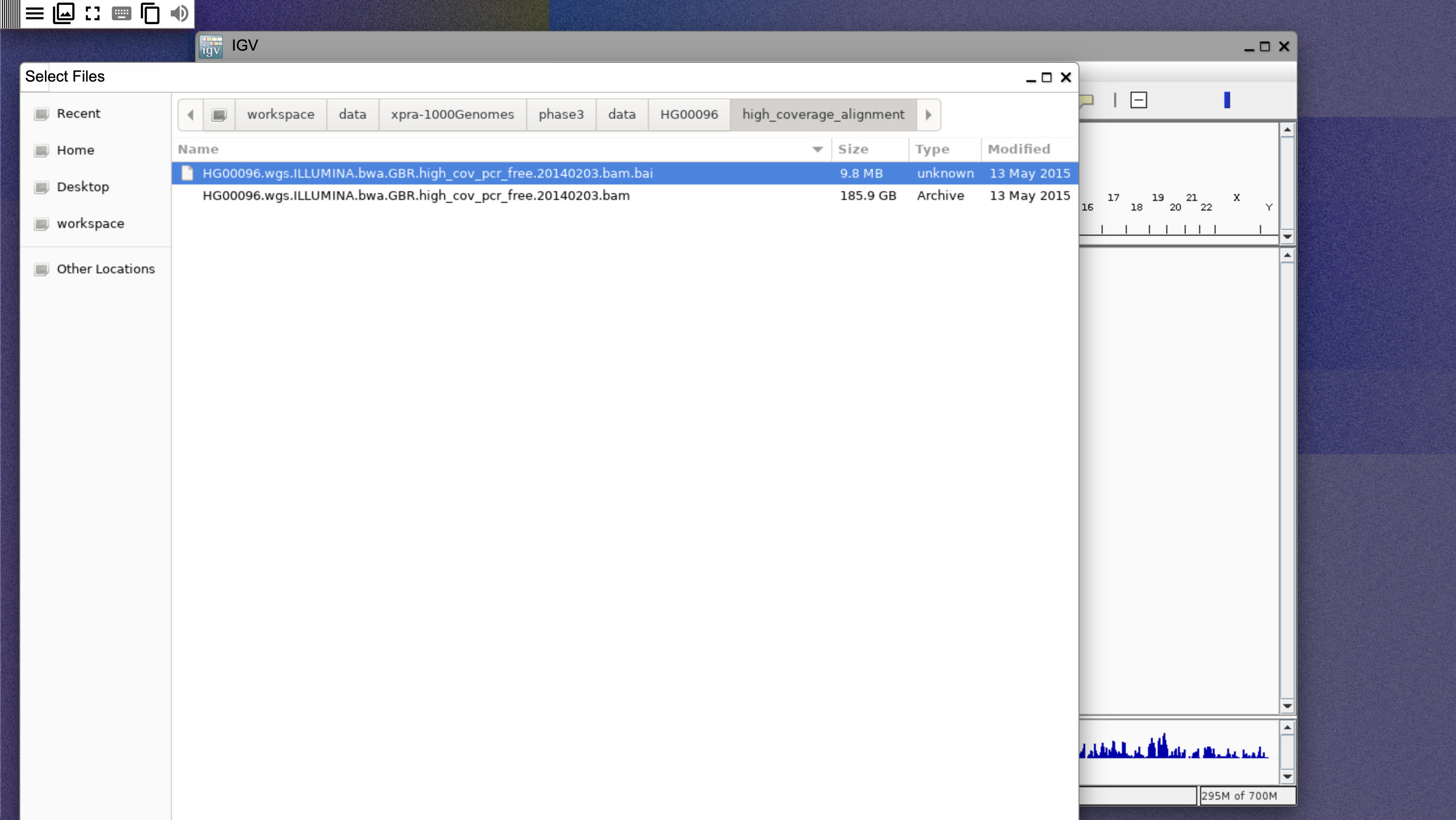
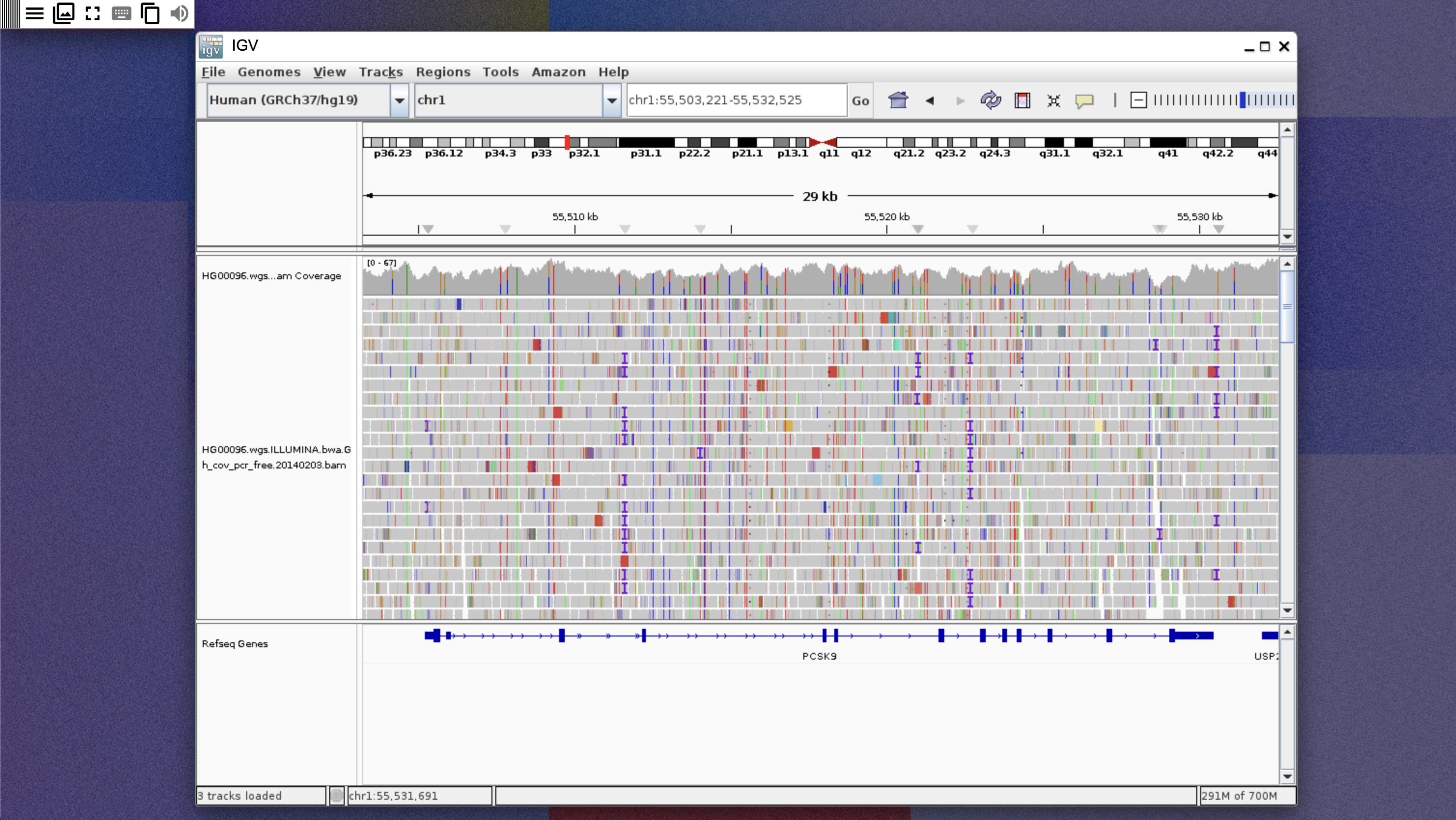
- Search for PCSK9 and zoom into one of the exons of the gene. A coverage graph and reads are shown, as below:
VS Code: Develop Nextflow pipelines
VS Code Studios give you a portable, interactive Nextflow development environment. The template includes the Nextflow VS Code extension, which uses the Nextflow language server to provide syntax highlighting, code navigation, code completion, and diagnostics for Nextflow scripts and configuration files. In this example, you add Conda and nf-core tools, run nf-core/fetchngs with its test profile, and scaffold a new pipeline with the nf-core template.
Create the VS Code Studio
-
From the Studios tab, select Add Studio.
-
In the Compute & Data tab:
- Select your AWS Batch compute environment.
- Allocate at least 4 CPUs and 16384 MB RAM.
- Mount the NGI iGenomes bucket you added with Data Explorer, plus any data directories you need for your own pipelines. The nf-core/fetchngs
testprofile uses the NGI iGenomes public data.
-
In the General config tab:
-
Select the latest VS Code container image template from the list.
-
Optional: Enter a unique name and description for the Studio.
-
Check Install Conda packages and paste the following into the YAML textfield:
channels:
  - conda-forge
  - bioconda
  - anaconda
dependencies:
  - nf-core
  - conda
-
-
Select Add and start, then select Connect in the options menu to open the session in a new browser tab when it is running.
-
Inside the Studio session, run
code .to use the clipboard.
See User and workspace settings to import your existing VS Code configuration and preferences into the session.
Run nf-core/fetchngs with Conda
Run the following command in the session terminal:
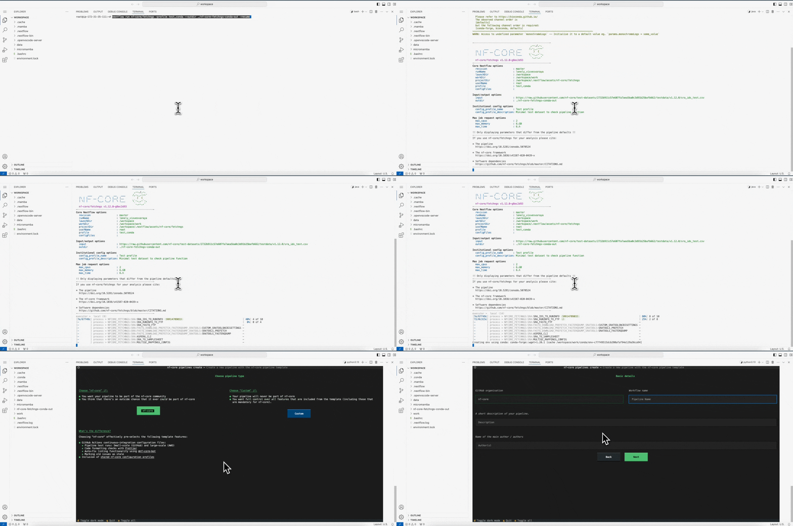
nextflow run nf-core/fetchngs -profile test,conda --outdir ./nf-core-fetchngs-conda-out -resume
Write a Nextflow pipeline with nf-core tools
- Run
nf-core pipelines createto create a new pipeline. Choose which parts of the nf-core template you want to use. - Run
code <your new pipeline>to open the new pipeline as a project in VS Code and develop it with the help of the Nextflow language server and nf-core tools.
Share a session with collaborators
To share a running Studio session with collaborators inside your workspace, select the options menu for the session, then select Copy Studio URL. Other authenticated workspace users can use this link to access the session directly and collaborate in real time.
Stop and manage your sessions
A Studio session runs — and consumes compute resources — until you stop it or it encounters a technical issue. To stop, restart, or inspect the configuration of your sessions, see Manage Studios.
Next steps
- Custom environments: Add Conda packages to a Seqera-provided image or bring your own container image.
- Example custom Studios: Ready-to-use Dockerfiles and pre-built images for Marimo, Streamlit, CELLxGENE, Shiny, and more.
- Add a Studio from a Git repository: Build a Studio directly from a repository that contains a Dockerfile.
- Studios troubleshooting: Fixes for common session and build issues.